Interpretable Machine Learning - Model-Agnostic Methods - (1) Partial Dependence Plot (PDP)

Overview

After all those interpretable models, we now go forward to model-agnostic methods. One obvious merit among many pros is that model-agnostic methods do not depend on the model type we’re interested in. Ribeiro et al.¹ claims that there should be three desirable aspects of a model-agnostic explanation system:

• Model flexibility: independence on the models.
• Explanation flexibility: should not be limited to one form of explanation.
• Representation flexibility: should have various feature representation methods to effectively explain the model in certain domain.

Partial Dependence Plot

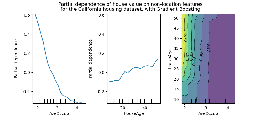
Partial dependce plot using scikit-learn for California Housing Dataset.

PDP (or PD plot), for short, is one of the premitive method to see the effects of one or two features, suggested by Friedman². The partial dependence function for regression is defined as:

\[\hat{f}_{x_S} (x_S) = \mathbb{E}_{x_C} \hat{f} (x_S, x_C) = \int \hat{f} (x_S, x_C) dP(x_C) \approx \frac{1}{n} \sum_{i=1}^n \hat{f} (x_S, x^{(i)}_C)\]

Here, $x_S$ is the set of features we are interested in (usually one or two), and $x_C$ consists of all other complement features. $\hat{f}$ represents the model. Since the exact expectation is only theoretically calculable, we estimate the marginalised model by Monte Carlo method, as stated in the last term above.

An assumption of the PDP is that the features in $C$ are not correlated with the features in S. If this assumption is violated, the averages calculated for the partial dependence plot will include data points that are very unlikely or even impossible.

For classification where the machine learning model outputs probabilities, the partial dependence plot displays the probability for a certain class given different values for feature(s) in $S$. An easy way to deal with multiple classes is to draw one line or plot per class.

PDP is a global method: The method considers all instances and gives a statement about the global relationship of a feature with the predicted outcome.

Categorical features

So far, we have only considered numerical features. For categorical features, the partial dependence is very easy to calculate. For each of the categories, we get a PDP estimate by forcing all data instances to have the same category. For example, if we look at the bike rental dataset and are interested in the partial dependence plot for the season, we get 4 numbers, one for each season. To compute the value for “summer”, we replace the season of all data instances with “summer” and average the predictions.

Pros and cons

Pros

The computation of partial dependence plots is intuitive: The partial dependence function at a particular feature value represents the average prediction if we force all data points to assume that feature value.

If the feature for which you computed the PDP is not correlated with the other features, then the PDPs perfectly represent how the feature influences the prediction on average. In the uncorrelated case, the interpretation is clear: The partial dependence plot shows how the average prediction in your dataset changes when the $j$-th feature is changed. Note that this merit remains only in the uncorrelated situation.

Partial dependence plots are easy to implement.

The calculation for the partial dependence plots has a causal interpretation. We intervene on a feature and measure the changes in the predictions. In doing so, we analyze the causal relationship between the feature and the prediction.³ The relationship is causal for the model – because we explicitly model the outcome as a function of the features – but not necessarily for the real world!

Cons

The realistic maximum number of features in a partial dependence function is two. This is not the fault of PDPs, but of the 2-dimensional representation (paper or screen) and also of our inability to imagine more than 3 dimensions.

Some PD plots do not show the feature distribution. Omitting the distribution can be misleading, because you might overinterpret regions with almost no data. This problem is easily solved by showing a rug (indicators for data points on the x-axis) or a histogram.

The assumption of independence is the biggest issue with PD plots. It is assumed that the feature(s) for which the partial dependence is computed are not correlated with other features. For example, suppose you want to predict how fast a person walks, given the person’s weight and height. For the partial dependence of one of the features, e.g. height, we assume that the other features (weight) are not correlated with height, which is obviously a false assumption. For the computation of the PDP at a certain height (e.g. 200 cm), we average over the marginal distribution of weight, which might include a weight below 50 kg, which is unrealistic for a 2 meter person. In other words: When the features are correlated, we create new data points in areas of the feature distribution where the actual probability is very low (for example it is unlikely that someone is 2 meters tall but weighs less than 50 kg). One solution to this problem is Accumulated Local Effect plots or short ALE plots that work with the conditional instead of the marginal distribution.

Heterogeneous effects might be hidden because PD plots only show the average marginal effects. Suppose that for a feature half your data points have a positive association with the prediction – the larger the feature value the larger the prediction – and the other half has a negative association – the smaller the feature value the larger the prediction. The PD curve could be a horizontal line, since the effects of both halves of the dataset could cancel each other out. You then conclude that the feature has no effect on the prediction. By plotting the individual conditional expectation curves instead of the aggregated line, we can uncover heterogeneous effects.

note: this post is almost identical to the Molnar’s original page. Refer his page for the examples.