Interpretable Machine Learning - Interpretable Models - (1) Linear Regression

Here I skip the definitions and some qualitative concerns for the interpretability and move on to the interpretable models from Molnar’s reference¹. The models introduced in this post are more like statistically founded approaches, which means they might not be able to applicable to complex tasks such as speech recognition or object detection. Nevertheless, first things first. Here I introduce 6+ ‘classical’ models for classification and regression.

Algorithm	Linear	Monotone	Interaction	Classification	Regression
Linear regression	O	O	X	X	O
Logistic regression	X	O	X	O	X
Decision trees	X	?	O	O	O
RuleFit	O	X	O	O	O
Naive Bayes	X	O	X	O	X
k-NN	X	X	X	O	O

A table from Interpretable Machine Learning, Molnar(2021)¹.

Here, each criterion stands for:

• Linear: whether the association between features and target is linear
• Monontone: whether the change in the feature space always monotonically affects the target
• Interaction: whether the model innately consists of interactive features

Linear regression

The structure genrerally follows the Molnar’s page, but I added some insights from the ETHZ Computational Statistics’ lecture notes.

Formalisation

The classic. Linear regression is the simplest model which predicts the target as a weighted sum of the feature inputs. Let’s do a quick recap of the process. Denote the target values $\mathbf{y} \in \mathbb{R}^n$ and the features $\mathbf{X} \in \mathbb{R}^{n \times p}$ including interceptions. With the intractable noise $\mathbf{\epsilon}$, we assume the latent relationship:

\[y_i = \beta_1 x_{i,1} + \cdots + \beta_p x_{i,p} + \epsilon_i,\ \forall i \in [n]\]

or

\[\mathbf{y} = \mathbf{X} \mathbf{\beta} + \mathbf{\epsilon}\]

and aproximate the weight vector $\mathbf{\beta}$ with:

\[\hat{\beta} = \arg\min_{\mathbf{b}} \sum_{i=1}^{n} (y_i - \mathbf{x}_i^\intercal \mathbf{b})^2 = \arg\min_{\mathbf{b}} (\mathbf{Y} - \mathbf{X} \mathbf{b})^\intercal (\mathbf{Y} - \mathbf{X} \mathbf{b}) = (\mathbf{X}^\intercal \mathbf{X})^{-1} \mathbf{X}^\intercal \mathbf{Y}\]

Pretty straightforward, isn’t it? Also, if we assume all the noise are drawn from the i.i.d. normal distribution, i.e., $\epsilon_i \sim \mathcal{N}(0, \sigma^2)$, then we also can approximate $\sigma^2$ with

\[\hat{\sigma^2} = \frac{1}{n-p} \sum_{i=1}^n (y_i - \mathbf{x}_i^\intercal \hat{\beta})^2 \sim \frac{\sigma^2}{n-p} \chi^2_{n-p}\]

and can derive the distribution of $\hat{\beta}$:

\[\hat{\beta} \sim \mathcal{N}_p ( \mathbf{\beta}, \sigma^2 (\mathbf{X}^\intercal \mathbf{X})^{-1})\]

Note that linear regression looks elegant, but it bases heavy assumptions for the data which are listed below:

• Linearity between the features and the target.
• Normality of the features for the confidence interval of each weight (which will be shown later)
• Homoscedasticity (constant variance) of the error terms.
• Independence among the data points.
• Fixed features, which means the data points are not variables but given constants.
• Absence of multicollinearity, which means the independence among the features.

Model selections

If there are too many features, we might want to reduce the dimension of the feature spaces while we don’t lose the predictive power or any other performance measure. There are majorly three ways to do so: subset selection, shrinkage, and dimension reduction (i.e., principal component analysis). The last one is hard to interpret, so let’s concentrate on the rests.

• Subset selection

When we want select only $q$ features from the data, the best way to do this is to consider $\binom{p}{q}$ models and choose the “best” model among those. However, this approach is computationally heavy, so we often do the greedy approaches in either forward or backward direction to choose the models among the limited scopes. This field is not dead yet - you can see the presentation pdf for the seminar handled this topic in here, if you’re interested in :)

Here, we often choose the criteria of the “best” model from Akaike Information Criterion (AIC), Bayesian Information Criterion, or adjusted R-squared, which will be explained later.

• Shrinkage

Two veins of the shrinkage methods are prevailing: Lasso and Ridge. Those are often called as regularisation techniques as well, as they regularise the L1-norm and L2-norm of the weights $\beta$, respectively. With attaching the regularising term on the objective function with the scale parameter $\lambda$, Ridge regression on the standardised data can be explicitly written:

\[\hat\beta^{Ridge} = (\mathbf{X}^\intercal \mathbf{X} + \lambda \mathbf{I})^{-1} \mathbf{X}^\intercal \mathbf{y},\]

but Lasso only have numerical solutions via least angle regression (iterative algorithm) or so.

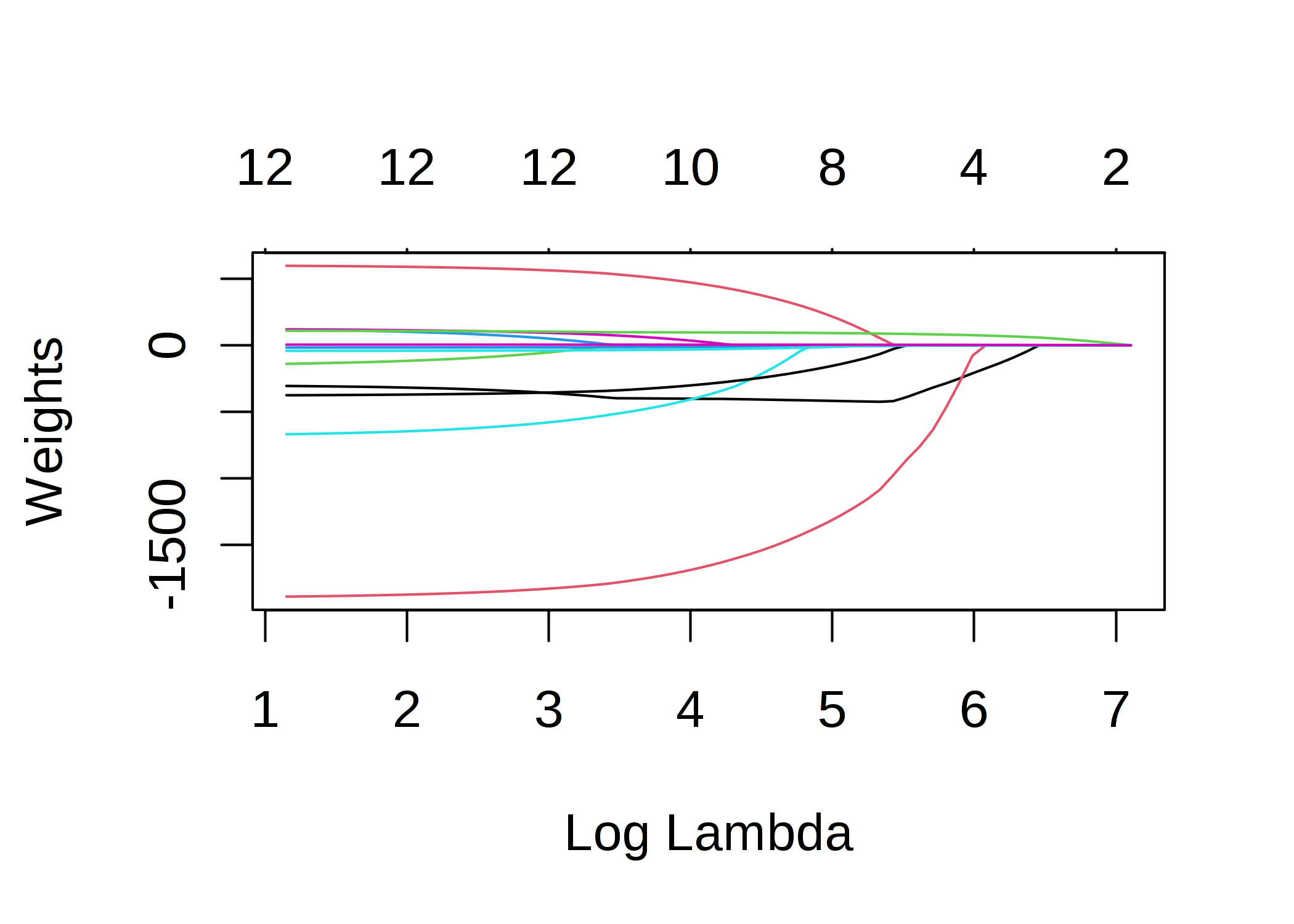
Lasso regression’s feature weights vs $\lambda$. Note that the more weights goes zero as $\lambda$ grows.

The funny thing here is that while Ridge still shows the continuous weights among all the features, Lasso regression innately “selects” the important features when the regularisation parameter $\lambda$ is big enough. From this property, we can shrink the model size based on the importance of each feature.

Interpretation

• Weights $\beta$

We can interpret the results of the linear regression: for $k$-th feature, $x_{\cdot, k}$, $\hat\beta_k$ is the expectation of the result gap of the two inputs share all the features but differ in $k$-th with 1. You can derive it easily by the linearity. This interpretation holds for both numerical features and categorical features.

Also, the feature importance of $x_k$ is measured by the absolute value of the t-statistic:

\[t_{\hat\beta_k} = \frac{\hat\beta_k}{se(\hat\beta_k)},\]

where $se$ is the standard error.

• R-squared measurement

R-squared or $R^2$ is the measurement represents the portion of variance in $y$ that is explained by the linear regression model. It is defined as:

\[R^2 = 1 - \frac{RSS}{TSS},\]

where

\[RSS = \sum_{i-1}^n (y_i - \hat{y}_i)^2,\ TSS = \sum_{i=1}^n (y_i - \bar{y}_i)^2\]

RSS stands for the residual sum of squares and TSS is for total sum of squares. Each of term can be interpreted as following: $RSS/(n-1)$ is the sample variance of the residuals $\epsilon_1, \cdots \epsilon_n$, and $TSS/(n-1)$ is the sample variance of the data labels $y_1, \cdots y_n$. Hence, $RSS/TSS$ should be low if the model works well, which directly implies that the higher $R^2$ is, the better the model is.

Here, we can also consider the adjusted R-squared to take account of the number of features $p$:

\[R^2_{adj} = 1 - \frac{RSS/(n-p)}{TSS/(n-1)}\]

• Confidence intervals

Confidence interval with the confidence $C$ means that the estimator will have the value within the interval with the probability $C$. I won’t go through the technical details of the derivation for those formulas, but it’s worth to mention the full forms. As it is known that

\[\frac{\hat\beta_k - \beta_k}{se(\hat\beta_k)} \sim t_{1-\alpha/2,\ n-p},\]

we can say $(1-\alpha) \cdot 100$% confidence interval for $\beta_k$ is

\[CI(\beta_k, (1-\alpha) \cdot 100) = \hat\beta_k \pm se(\hat\beta_k) \cdot t_{1-\alpha/2, n-p}.\]

The range terms consist of the point estimate, the estimated standard error of the point estimate, and the quantile of the relevant distribution. This format holds for the other confidence intervals. For example, consider the new data $\mathbf{x}_0$. The confidence intervals for $\mathbb{E} y_0$ and $y_0$ are:

\[CI(\mathbb{E} y_0, (1-\alpha) \cdot 100) = \mathbf{x}_0^\intercal \hat\beta \pm \hat\sigma \sqrt{\mathbf{x}_0^\intercal (\mathbf{X}^\intercal \mathbf{X})^{-1} \mathbf{x}_0} \cdot t_{1-\alpha/2,\ n-p},\] \[CI(y_0, (1-\alpha) \cdot 100) = \mathbf{x}_0^\intercal \hat\beta \pm \hat\sigma \sqrt{1+\mathbf{x}_0^\intercal (\mathbf{X}^\intercal \mathbf{X})^{-1} \mathbf{x}_0} \cdot t_{1-\alpha/2,\ n-p}.\]

Pros and cons on interpretability

So far we took a look for the linear regression and how we interpret the results from the algorithm. Here, we summarise the merits and drawbacks of the linear regression in the eyes of interpretability. Based on the criteria on the Human-Friendly Explanations,

• Explanations are contrastive: YES, but has limitation on the highly unrealistic setting of standardised data points.
• Explanations are selected: NO, because the model does not select from the other options. Linear regression just calculate the weights by the formulas.
• Explanations are truthful: YES. As long as the data is nicely prepared, no other term can interfere the calculation during the inference time.
• Explanations are general and probable: YES. So clear mathematical foundations.

Other criteria relate on the social aspects, so we can say it depends on the interpreter of the resulting model.

Hence, long story short, linear regression generally works well, but only on the specific settings and assumptions. Keep in mind that this is the simplest form, and statistics community has already developed Generalised Linear Models (GLM) or Generalised Additive Models (GAM) to mitigate the weakness of the vanilla linear regression. I do not have a plan to go deeper for those topics, so pleas refer Molnar’s explanation on it here.