Interpretable Machine Learning - Interpretable Models - (2) Decision Tree

Logistic regression and GLM are somehow direct extension from the linear regression so I skip the post about those. Instead, in this post, we will take a look for another simple yet powerful method, decision tree. After we go through the basic of the decision tree, we will also take a look for the paper named “Neural-Backed Decision Trees”, which proposes the hybrid approach of decision tree and neural network.

Decision trees

The name itself of decision tree says quite much about the algorithm. Decision tree consists of a tree-like decision process and let the data follow the distinct route from the root to the terminal/leaf node. Each terminal node is classified as a single label.

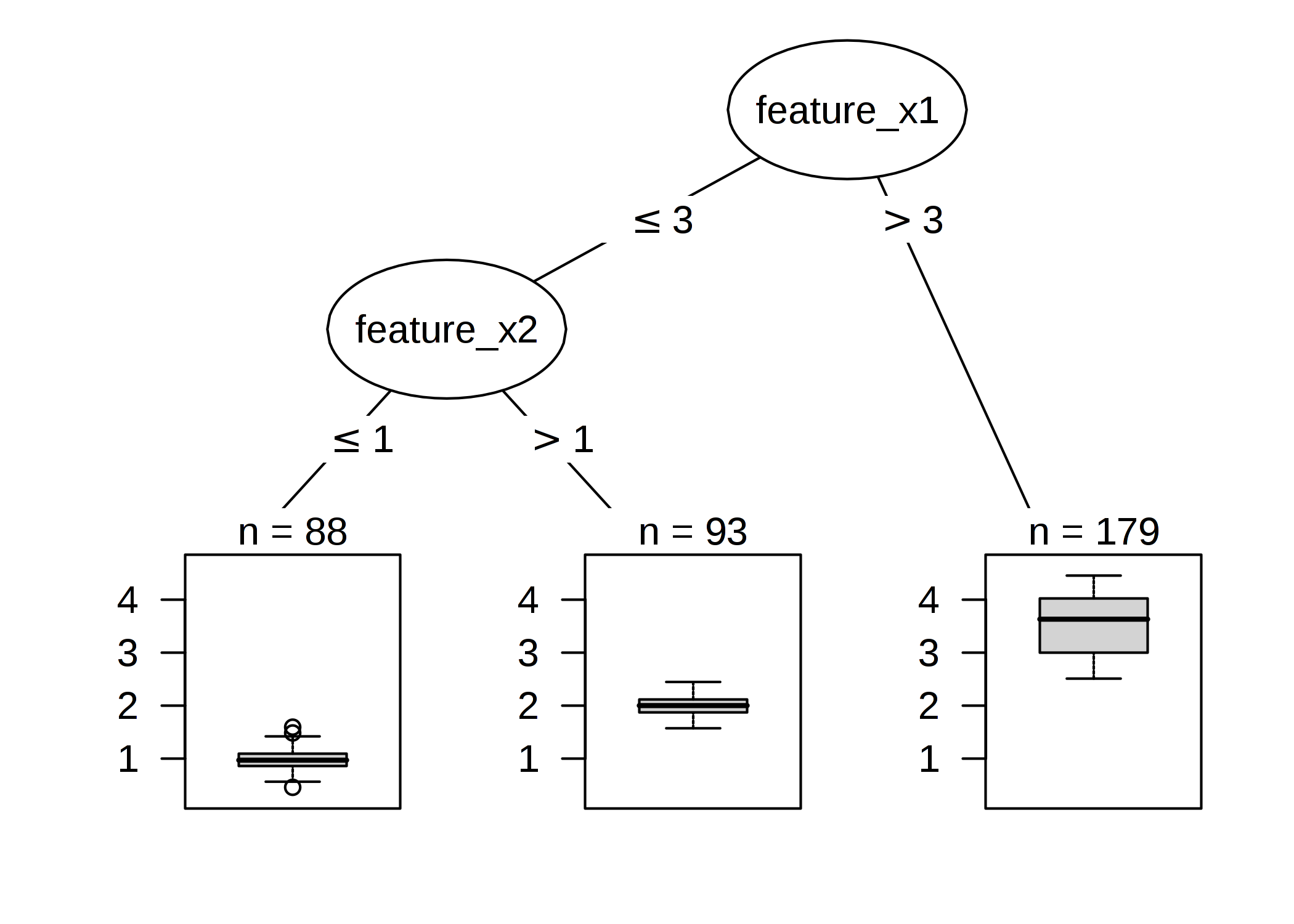
An example decision tree shape. Each intermediate node becomes the binary test statement to split the inputs into two mutually-excluive groups. Original image from Molnar’s page.

This is the formal statement of inference in the decision tree.

\[\hat{y} = \hat{f}(x) = \sum^{M}_{m=1} c_m I_{ \{ x \in R_m \} }\]

As mentioned earlier, each instance falls in to the unique leaf node($R_m$) with the class label (or the average value) of $c_m$. There are several algorithms to build a tree on a dataset, but let’s focus on CART (Classification and Regression Trees) algorithm in this post.

Building algorithm – CART

CART decides how to split the data based on the Gini impurity. Gini impurity given set is calculated by the sum of the multiplication of correctly classified probability ($p_i$) and wrongly classified probability ($\sum_{k \neq i} p_k = 1 - p_i$).

\[I_G(p) = \sum^J_{i=1} p_i \left( \sum^J_{k=1} p_k \right) = \sum^J_{i=1} p_i (1-p_i) = 1 - \sum^J_{i=1} p^2_i\]

Based on this measure, CART splits the given data by minimising the impurity of the resulting nodes. This applies both for the continuous and categorical features.

Interpretation

Interpretation of the decision tree is pretty simple: you only need to follow the conditions written on the intermediate nodes and make inference by the representative label of the terminal node where the instance eventually placed. Decision tree is the most human-friendly method to build the interpretable model and relatively fast to create the model.

In addition to the vanilla decision tree, we can extend the concept to random forest technique. This is out of scope of this post, but keep in mind that the extended method is the ensemble method with several decision trees on the subset of the dataset.

Pros and cons

Here goes the list of the pros of decision trees:

• Good for capturing interactions between features in the data. This is not quantitatibly done but by the interpreter’s signts.
• So easy interpretation even on the multidimesional data.
• Has natural visualisation.
• Creates good explanations. Following the route itself already produces natural explanations for the inference.
• No need of transformation of the features unlike the linear regression.

and cons:

• Fails to deal with linear relationships. Decision trees only split the data based on the step function. This eventually results in the lack of smoothness in the infefence. This can be alleviated by using oblique decision trees, the structure using non-orthogonal decision boundaries.
• Unstable structure. Even the slightest change in the training dataset can devastating change in the resulting tree. For the robust decision trees, check this out¹.
• The number of terminal nodes increases quickly with depth. The maximum number of leaves increases exponentially as the depth grows.

Neural-backed decision trees

As briefly shown before, decision trees are easy to build and easy to interpret, but certainly have their limitations. Wan et al.² wanted to maintain the good things from the decision trees for the concurrent models, so they designed NBDT; the hybrid approach of neural networks and decision trees to boost the interpretability of the high-end classifiers. Their intuitition is:

Neural-Backed Decision Trees (NBDTs) replace a network’s final linear layer with a decision tree. Unlike classical decision trees or many hierarchical classifiers, NBDTs use path probabilities for inference (Sec 3.1) to tolerate highly-uncertain intermediate decisions, build a hierarchy from pretrained model weights (Sec 3.2 & 3.3) to lessen overfitting, and train with a hierarchical loss (Sec 3.4) to significantly better learn high-level decisions (e.g., Animal vs. Vehicle).

Inference

Let $W \in \mathbb{R}^{d \times k}$ be the weight matrix of the final fully-connected layer of the pre-trained neural network. Denote the row vector of $W$ as $w_i$.

1. Seed oblique decision rule weights with neural network weights. Fix the structure of the decision tree shape with the complete binary tree, and allocate the row vectors $w_i$ to each leaf node. For the intermediate nodes, set with the average weight vector of all the leaf nodes in the subtree rooted by that node, i.e., \(w'_i = \frac{1}{|L(i)|} \sum_{j \in L(i)} w_j\)
2. Compute node probabilities. For each sample $x$, node $i$, and its child $j \in C(i)$, \(p(j|i) = \texttt{Softmax}(n_i^{\intercal} x) [j], \text{ where } n_i = (w_j^{\intercal} x)_{j \in C(i)}.\)
3. Pick a leaf using path probabilities. Denote the next traversal node of $i$ as $C_k(i)$ on the existing path $P_k$. Then $C_k(i) \in P_k \cap C(i)$. The probability of the leaf node labeled $k$ is: \(p(k) = \prod_{i \in P_k} p(C_k(i) | i).\) After that, the final class prediction $\hat{k}$ is calculated as the argmax of all the leaf node probabilities.

The authors claim that this approach is the “soft” decision process as all the leaf nodes are considered in probabilistic way, and more robust to the early mistakes happening on the shallow nodes.

Building induced hierarchies

After it, the author takes the strategy to build hierarchy structure by clustering algorithm based on the normalised assigned weights, $w_k / |w_k|_2$. The implementation shows they applied k-nn clustering for this.

Labeling decision nodes with WordNet

Then they labeled each intermediate nodes by finding the common ancestor of two nodes in the WordNet. This is for semantically plausible purpose for the interpretation.

Fine-tuning with tree supervision loss

They suggested a new loss named tree supervision loss by combining the original cross entropy loss for the classification and the additional term of cross entropy on the $p(k)$. The weights for each term changes along the training stage.

Results

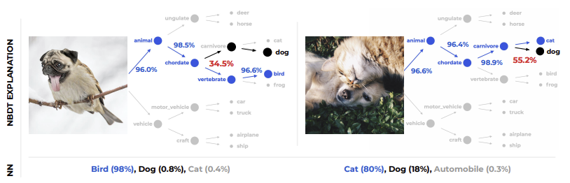
Types of ambiguous labels. NBDT explains which node is ambiguous and not.

Overally, NBDT shows impressive results. They showed that with the very slight drop of accuracy, NBDT produces much reasonable explanations for the predictions. Since, as you know, there is no way to quantitatively measure the explanability, the authors performed several surveys to human pool, including above interesting experiments.

Wrap up

We took a look for the decision trees and their modern application, NBDT. This simple yet powerful method is still widely used in the field, so worth be acknowledged. As the authors of NBDT confessed, the method has a weak chain between the induced hierarchy and labeling it. It would be nice further research to make logical grips on that ambiguous part to make NBDT better.