Interpretable Machine Learning - Neural Network Interpretation - (1) Pixel Attribution (Saliency Maps)

(Can we skip to the good part) Yes, after a while, I decided to skip all those ‘classical’ stuffs of interpretable ML, and proceed to neural network analysis! I know, you and I all love neural networks, and thanks to Christoph, their NN part is exclusive to web so we can peek and learn from the extensive writings. I’ve been extremely busy with getting used to my work and that’s why this is the very first post in 2022. There were some sessions I made in my work, but they were mostly for internal use only, so please accept my apology for the late update:)

Pixel Attribution

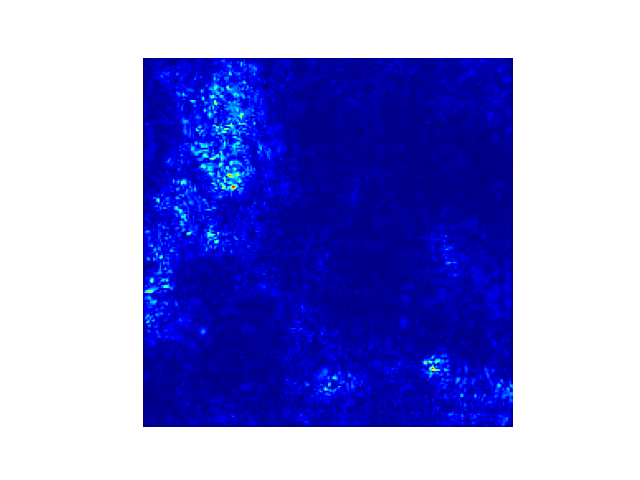
Saliency map example. The brighter a pixel is, the more significant it is.

The easiest and the most accessible field of the topic has always been computer vision. Pixel attribution, a special case of feature attribution in CV field, highlight the datapoints(pixels) which are relevant to a classification decision of a neural network. For general purpose feature attribution methods, we can refer SHAP, Shapley values, or LIME.

Consider a neural network having a logit dimension $C$. Denote the logit as $Z \in \mathbb{R}^C$ and the input image $x \in \mathbb{R}^p$. A feature attribution method is a function which maps $x$ into relevance scores for a single class, $c$ - $R_1^c, \cdots, R_p^c$. Although there are abundant amount of methods, but we can classify them into two major types:

1. Occlusion or perturbation based methods: those methods amend the input images to measure difference between the results. SHAP are LIME are the examples of this model-agnostic class.
2. Gradient based: those methods calculate gradients of each logit element with respect to the input features. Variations come from how those methods calculate the gradients.

Or, Christoph mentioned an alternative categorisation:

1. Gradient-only methods: those methods tell us whether a change in a pixel would change the prediction. The larger the absolute value of the gradient, the stronger the effect of a change of this pixel.
2. Path-attribution methods: those methods take a reference image or multiple images, such as an all-zero black image, to get the comparitive interpretation. Some path-attribution methods are “complete”, meaning that the sum of the relevance scores for all input features is the difference between the prediction of the image and the prediction of a reference image.

Let’s take a look at the popular methods of the linage. Have a good look at some example results of each method and go through the details.

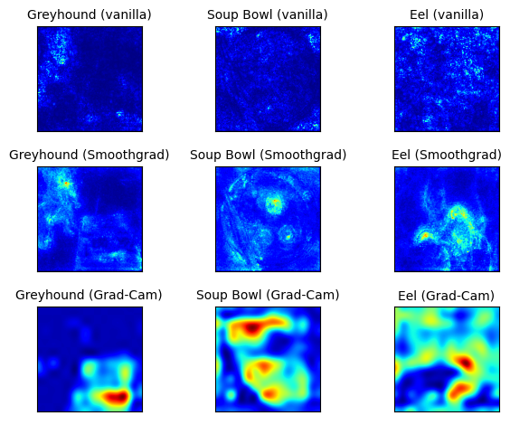
Examples of different pixel attribution methods.

Vanilla Gradient (Saliency Maps)

Vanilla Gradient¹ is the most basic method among the pioneer pixel attribution methods. We calculate the gradient of the loss function for the class we are interested in with respect to the input pixels. This gives us a map of the size of the input features with negative to positive values.

Briefly speaking, the steps of vanilla gradient goes like,

1. Perform a forward pass of the image of interest, $I_0$.
2. Compute the gradient of class score of interest with respect to the input pixels, $\nabla_{I} z_c = \frac{\delta z_c}{\delta I} |_{I=I_0}$.
3. Visualise the gradients.

Here, the method approximates the logic value as the first-order Taylor expansion: $z_c(I) \approx w^\top I + b$, where $w = \nabla_I z_c |_{I=I_0}$. However, it is ambiguous when the back-propagation encounters some non-trivial activations, such as ReLU. In that case, Vanilla Gradient handles it with:

\[\frac{\delta f}{\delta X_n} = \frac{\delta f}{\delta X_{n+1}} \mathbf{I}(X_n > 0)\]

, where $ReLU(X_n) = X_{n+1}$. What an elegant way to circumvent the issue! However, Vanilla Gradient has a saturation issue²; when ReLU is used, and when the activation goes below zero, then the activation is capped at zero and does not change any more.

To mitigate the saturation problem, DeconvNet² suggested a different way of calculating gradient than Vanilla Gradient - not checking the value of $X_n$ but seeing $X_{n+1}$ to put in the indication function. This reduces some gradient information loss during the back-propatagion.

Grad-CAM

Grad-CAM is another popular way of pixel attribution, particularly for convolutional neural networks. Unlike other methods, the gradient is not backpropagated all the way back to the image, but (usually) to the last convolutional layer to produce a coarse localization map that highlights important regions of the image. Christoph provides an intuitivie explanation of Grad-CAM. Long story short, Grad-CAM points out how each convolution filter focuses on the class of interest $c$ by ReLU’ing out other classes’ impact. Let’s go over the process step by step:

1. Forward pass an image through the CNN and get the logits.
2. Set all other class activations to zero.
3. Back-propagate the gradient of the class of interest to the last convolutional layer before the fully connected layers: $\frac{\delta z_c}{\delta A^k}$.
4. Weight each feature map “pixel” by gradient for the class: $\alpha^c_k = \frac{1}{const} \sum_{w,h} \frac{\delta z_c}{\delta A^k_{w,h}}$, the $const$ term is the normalisation constant for the global average pooling.
5. Calculate an average of the feature maps, weighted per pixel by the gradient.
6. Apply ReLU to the averaged feature map.

The resulting image will form a heatmap, which is not often quite precise compared to other methods. However, it still provides good intuitition of which place of the image is focused on during the inference time.

SmoothGrad

SmoothGrad³ is not a standalone method but an attachable part. This is pretty simple; just add some Gaussian noise on the original image and aggregate the gradients over several modified images! Nothing special, but it will result in more robust analysis compared to the single-shot.

Pros and Cons

For pros, those methods are visual, which means the practioner can easily understand what’s going on. Also, those methods are generally faster than model-agnostic methods.

Cons, however, are quite a lot more than pros. First, no one knows which method is ‘correct’. Also, Ghorbani et al.⁴ found that pixel attribution methods are quite fragile to adversarial examples. There are many issues over the trustworthiness of the metrics and visual interpretations as well.